UNSW-NB15使用CNN进行分类
前言
在UNSW-NB15数据集上进行基准测试实验,看下效果如何,以便后续进行调整
测试内容(未使用Gsmote平衡训练集)
- 对预处理后的数据集使用
CNN进行二分类 - 对预处理后的数据集
使用DNN进行二分类 - 对比二者的分类效果
数据预处理
预处理内容
- 对
proto、service、state三个全是字符型值的列进行one-hot编码 - 将训练集和测试集在同一标准下进行归一化
- 删除
attack_cat列
预处理代码
1 | def load_data(): |
实验结果
CNN二分类
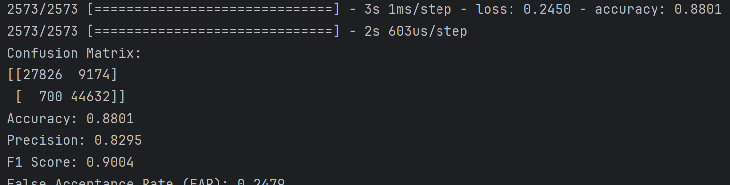
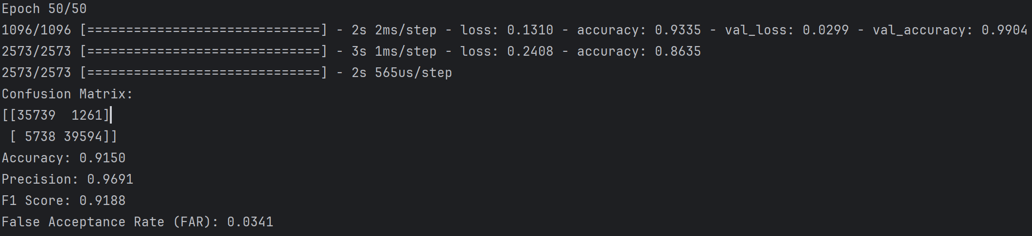
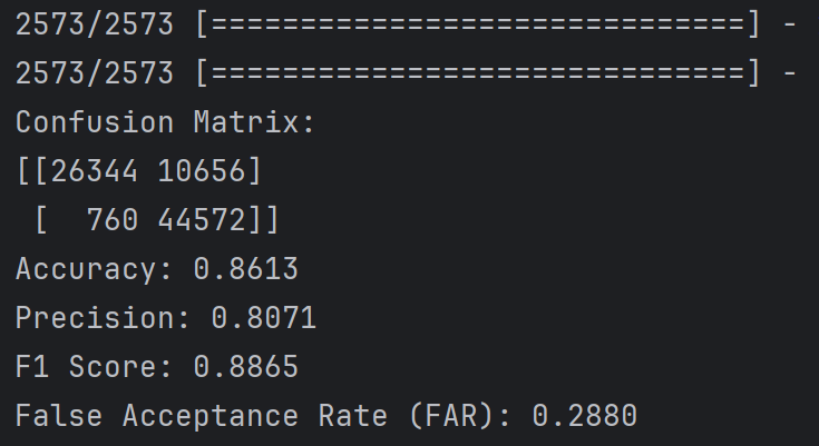
阈值为0.5时的实验结果如下
阈值为0.5,learning_rate=0.001,epochs=50,batch_size=128
效果不好,有很多正常样本误报为攻击样本,有11763个正常样本被判断为了攻击样本,假阳性很高;

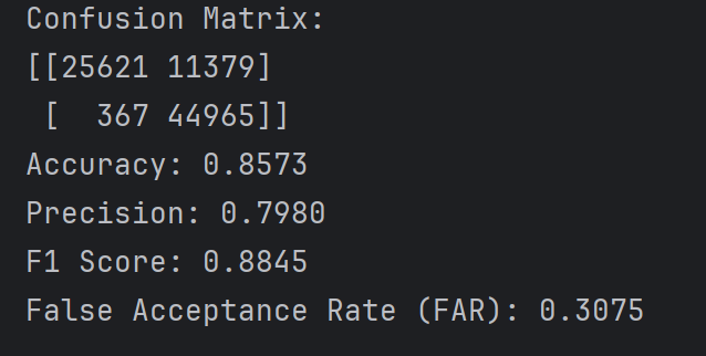
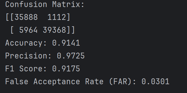
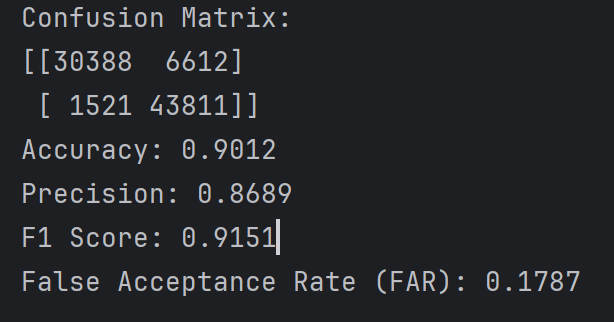
第二次测试效果比第一次好很多,很奇怪

第三次又恢复原样了,炼丹太玄学了
第四次,结果又变成和第一次一样烂了
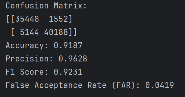
阈值为0.9时的实验结果如下
可以看到各项评估指标都好了一点,但是很明显假阴性的样本多了不少,阈值为0.5时假阴性在300~1200范围内浮动,但是阈值设为0.9时一下子变成5700了,虽然假阳性样本从10000多变成了1200多(因为概率低于0.9的都算正常样本,可见有很多正常样本的最终预测概率在0.5~0.9之间),因为假阳性样本下降的数量大于假阴性样本上升的数量,所以各项指标都变好了,但实际并不代表模型效果变好了
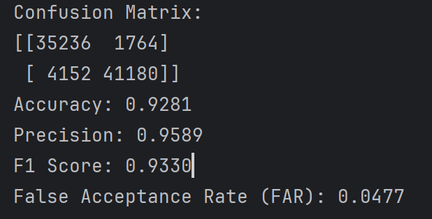
阈值为0.9时第二次测试
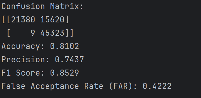
阈值为0.1时的实验结果如下
当阈值为0.1时,会导致很多正常样本被划分为攻击样本,即假阳性很高(15620个,比之前阈值为0.5的11000多了四千个),因为概率只要大于0.1就当作攻击样本,但是还有21380个正常样本实际预测概率实际上是小于0.1的,从这个角度看预测准度还是挺不错的
DNN二分类
阈值为0.5时的实验结果如下
在UNSW-NB15使用CNN的效果好像比CNN要好一点
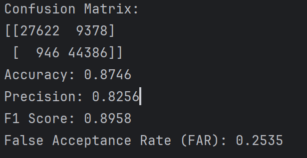

第四次 算是比较好的结果了,偶尔能出一次这种结果,玄学
阈值为0.9时实验结果如下
这个倒是和CNN差别不大,误差也挺小,但是阈值0.5差距蛮大
和第上一次结果差不多

第三次 和上两次大差不差
阈值选择问题
正常二分类都使用0.5作为阈值,但是可以根据需要自定义调整阈值,阈值不同最后的结果也不一样
在二分类问题中,预测模型输出的值通常是一个介于0和1之间的概率,表示样本属于正类的信心程度。阈值决定了将这个概率转换为具体类别的界限。如果概率大于0.5,预测为正类(1,即攻击样本);否则预测为负类(0,即正常样本)。这是一种常见的默认选择,适用于类别分布相对均衡的情况。
阈值等于0.5
在这个设置下,模型对正类和负类的识别相对平衡,但存在一定的假阳性(FAR较高),表明一些正常流量被误判为攻击
阈值大于0.5
在这个设置下,模型的精确率大幅提高,意味着大部分预测为攻击的样本确实是攻击。这降低了假阳性率(FAR显著降低),但假阴性(即真实攻击被误判为正常)增加
高阈值的优缺点
高阈值的优点:提高了精确率,减少了假阳性(FAR显著降低),适合对误报敏感的场景。
高阈值的缺点:可能导致更高的假阴性数量,错过一些实际的攻击。因为概率为0.9时才当作是攻击样本,概率低于0.9都当作正常样本,所以导致会错过比较多的实际攻击,假阴性更高了
模型代码
CNN代码
1 | import pandas as pd |
DNN代码
1 | import pandas as pd |